A few words about CLASSIFICATION
Table of Contents
1. Classification, clustering and variables
2. Statistical learning, machine learning and evaluation of the results
3. SL: Linear regression, logistic regression and discriminant analysis
4. ML: Random forests and SVM
5. Examples with R
1. Classification, clustering and variables
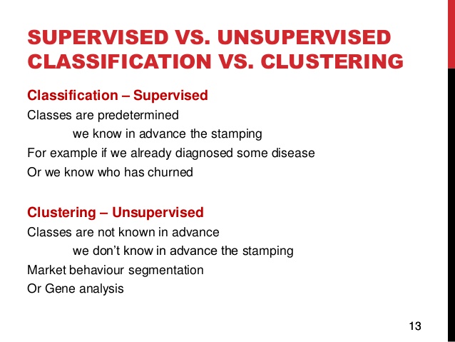
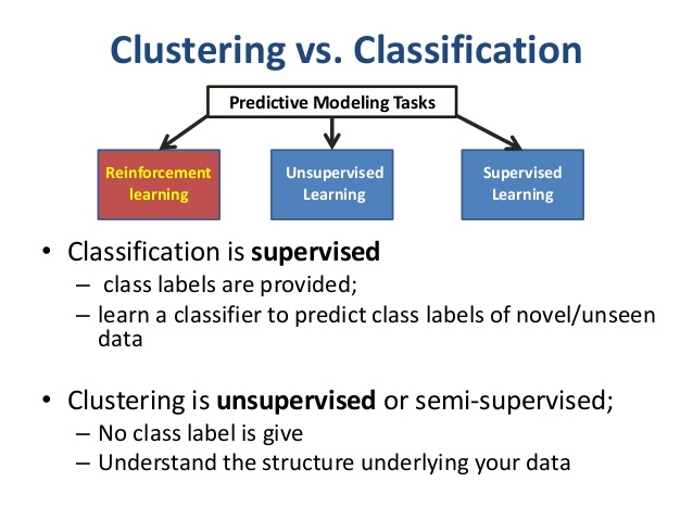
In the context of statistics, to perform a classification, you must have a fixed set of predefined classes and the objective is to know which class a new object belongs to. On the contrary, clustering tries to group a set of objects into clusters and to find whether there is some relationship between the objects. To define the "correct" number of clusters is in itself already a difficult problem. In the context of computer science (or machine learning), classification is called supervised learning and clustering is called unsupervised learning. With french words, one speaks of classification non supervisée and of classification supervisée or prédiction statistique.
Wiki references: classification en fr ; clustering en fr.
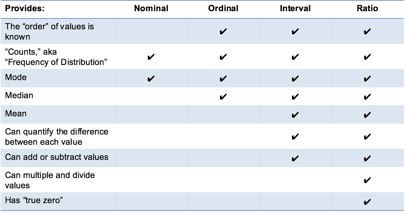
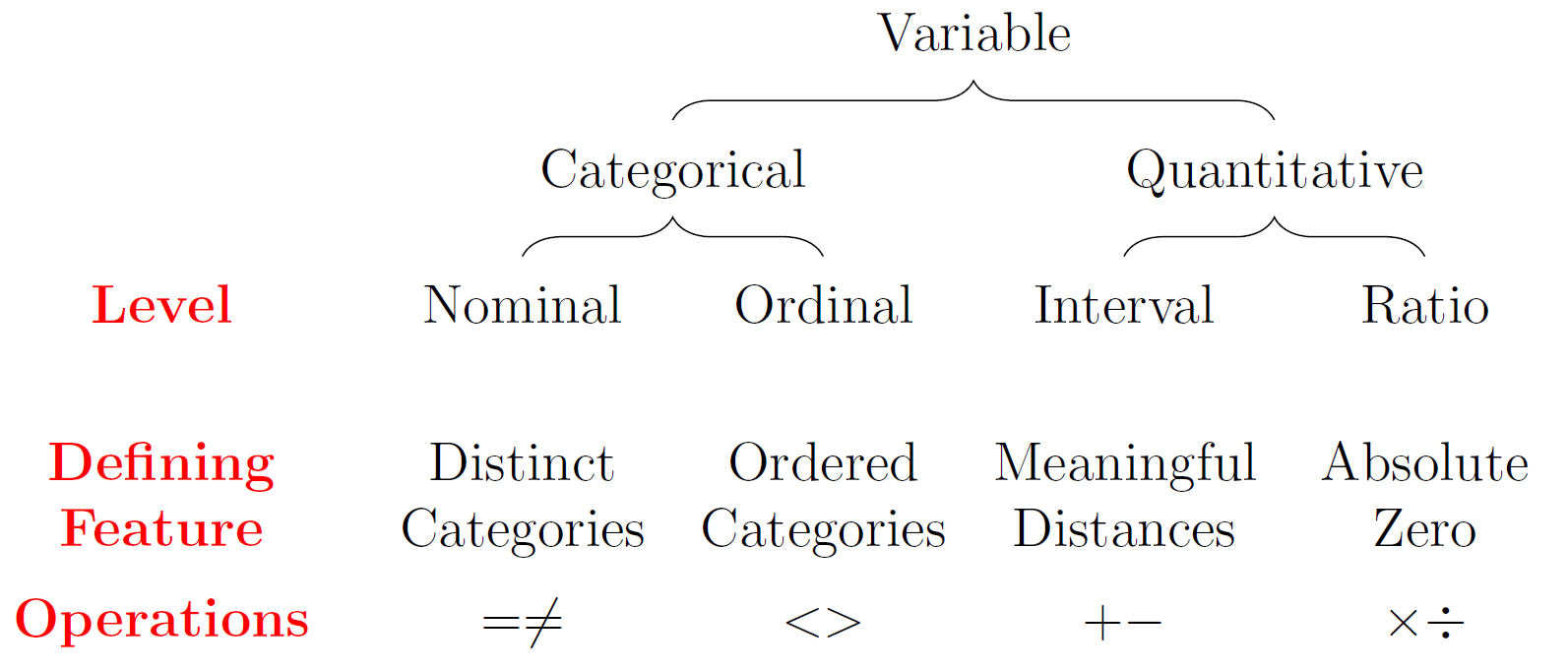
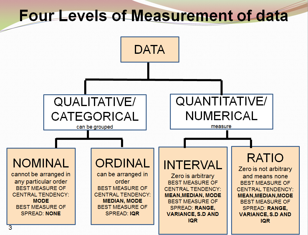
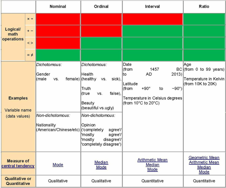
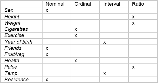
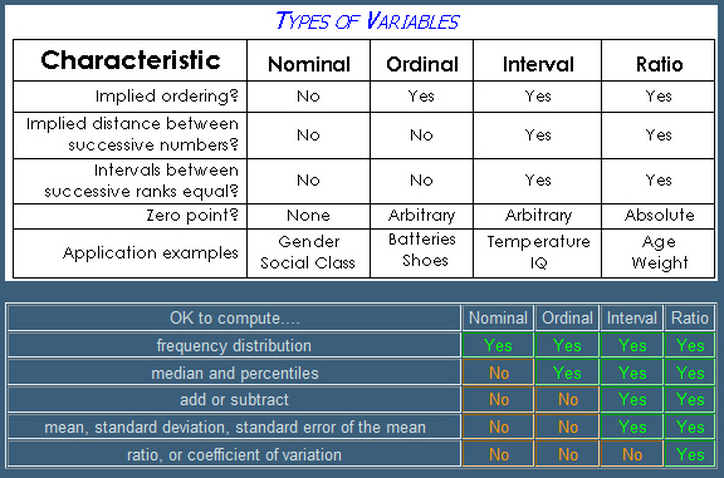
So from now on, we will be dealing only with classification since we have to predict pathogenicity in terms of degree, level, class, strength...Usually, the classes are defined by numerical values, such as 0,1 (binary clasification) or 1, 2, 3...n (multiclass classification). The interpretation of these values such as 1=good, 0=bad or 1=cat, 2=dog, 3=other is defined through labels. Statistically speaking, a column of values for a class is called a categorical variable (in French: variable qualitative). If there is a natural order, the variable is ordinal. Otherwise, it is nominal. The R software calls these variables factors and the values are named levels. It is usal to call the class variable the outcome or the target (cible or variable d'intérêt, in French). The other variables -- either discrete or continuous -- used in the dataset to determine or predict the classes, are called the predictors (prédicteurs, in French).
Links to understand the nature of a variable such as nominal vs interval: ucla graphpad nominal-ordinal-interval-ratio.
2. Statistical learning, machine learning and evaluation of the results
There is a small difference between the statistical and the computer science approaches. Statisticians use formulas and mathematical models. They are often interested by the explanation of the prediction, that is, to be able to quantify how predictors influence the value of the outcome. Computer scientist also allow themselves to use only predictive models (or "black boxes") via algorithms instead of formulas to compute values and coefficients, like neural networks for instance, just to have the correct outcomes even without knowing precisely how they are predicted and without looking back at the input predictors or trying to interpret the intermediate predictors that have been used.
Wiki links: predictive modelling en ; predictive analytics en fr.
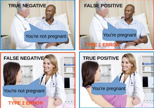
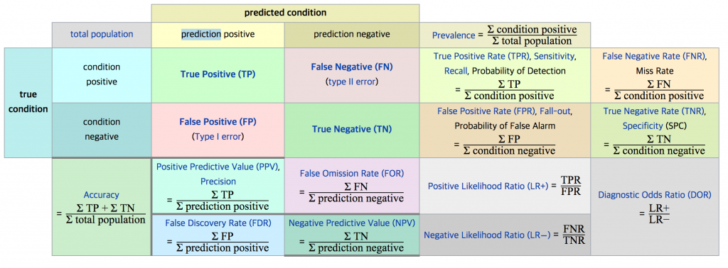
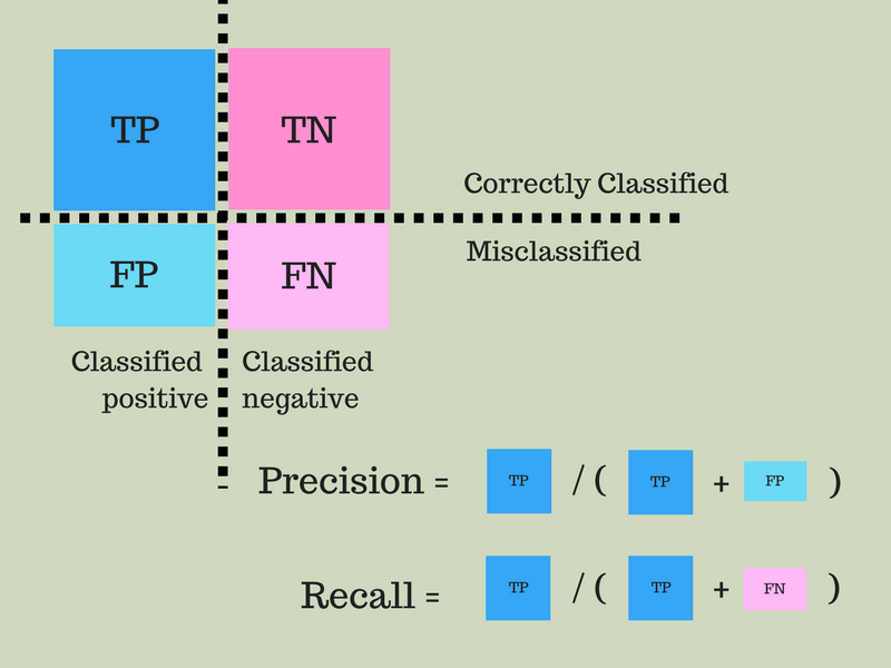
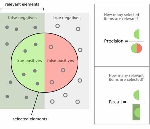
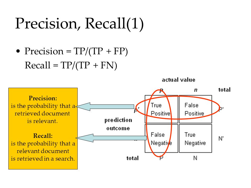
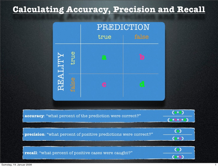
Once we have obtained the predicted values for the classes, there are classical ways to show and evaluate the capacity of the model to achieve a good prediction. Usually one uses data with known outcome to see if we are able to recover the original oucomes. First, the confusion matrix allows to see the number or percentages of correct and uncorrect predictions such as true positive and true negative for binary classes in the case of binary classification. Then, summing up these values and computing relative ratios, statistical indicators leads to indexes known as sensitivity, predictive power, precision, recall, TPR, FPR, ROC curve...
For definitions, see for instance PNPV. . For real computations, use my web page valeurs diagnostiques.
Links: precision/recall ; ROC curve ; sensibilité/spécificité
3. SL: Linear regression, logistic regression and discriminant analysis
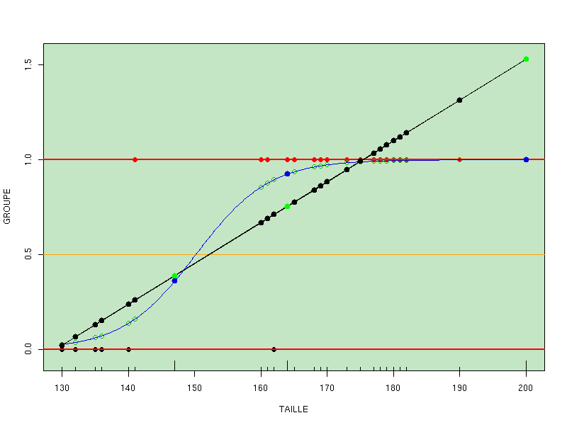
In mathematics, there is a lot of formulas and functions to produce y as f(x). In statistics, the classical way to produce y knowing some xi is to use a simple linear sum with coeffficients ci or βi, thus leading to classical linear regression. It can be generalized as GLM.
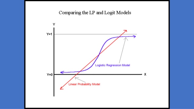
Let's deal first with binary classification, that is, we want 0 or 1 as the output. Since linear regression does not produce bounded values, it is not suitable for binary classification. But using a simple link function in GLM called logit one gets a prediction formula ranging from 0 to 1 for all input values, and a simple rule based on a threshold s (0 if prediction is less than s, 1 if it is greater than or equal to s) allows to have only two classes as a result. This is what is called binary logistic regression.
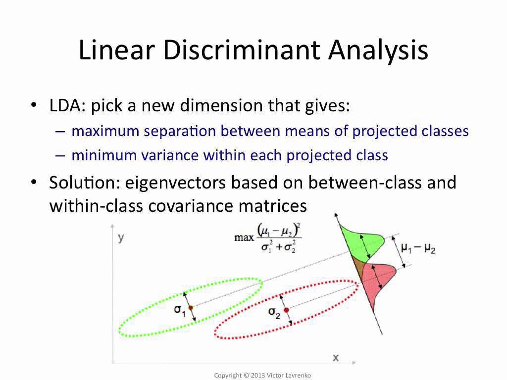
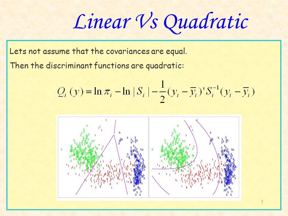
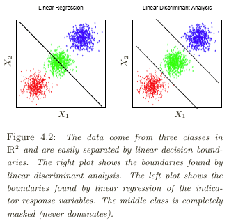
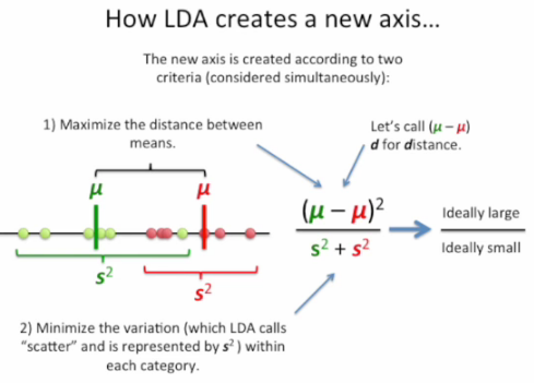
Let's have now more than two classes. It is possible to generalize the binary logistic regression to multinomial logistic regression if the outcome is not ordered, and to ordinal logistic regression in the other case. There is also an other family of methods called discriminant analysis that returns as output the probabilities of belonging to each outcome class. Depending on options, it can be a linear discriminant analysis (LDA) or a quadratic discriminant analysis (QDA).
Logistic regression methods are better explicative models than discriminant analysis ones because they assign coefficients to each input variable, thus giving the ability to understand the influence of each input variable. Moreover, LDA is related to PCA.
4. ML: Random forests and SVM
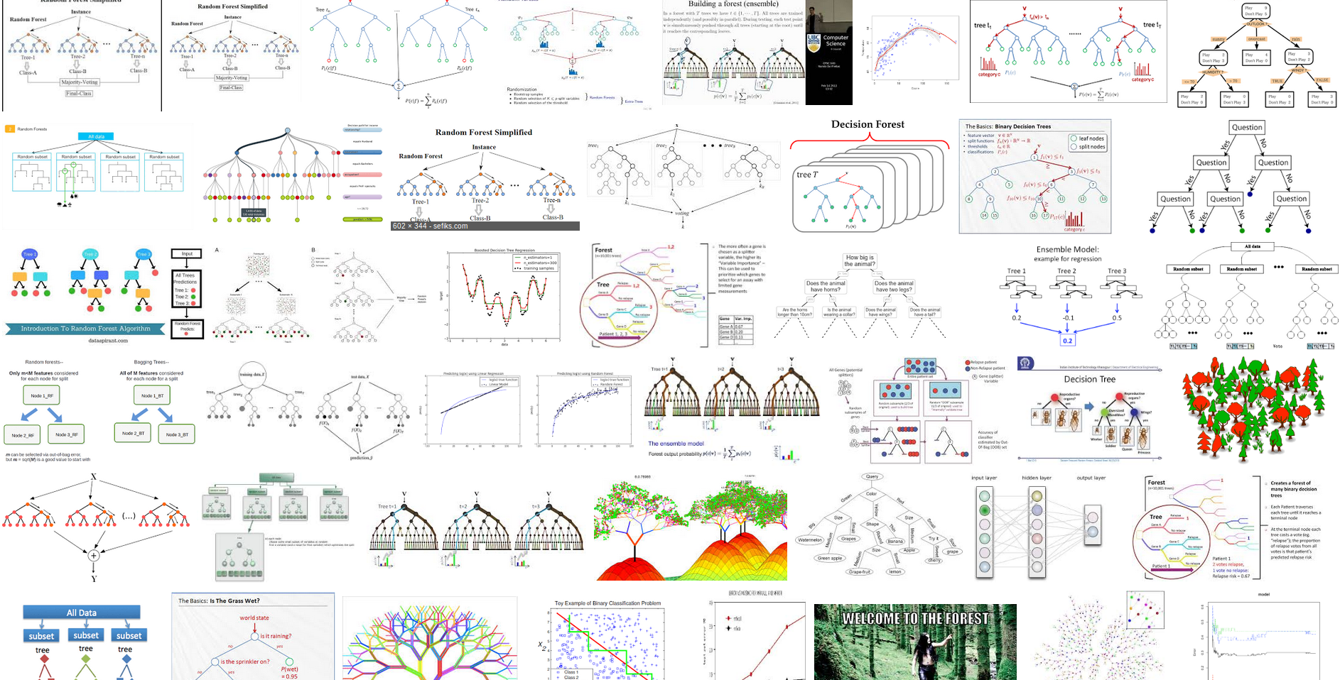
A random forest predictor uses in a bootstrapping way many many decision trees to build a classifier based on average, consensus, mode or majority vote computations. This means that it builds a lot of input datasets from the original one, using random sampling with replacement, to compute a lot of trees and then aggregates them. Even if there are some parameters to use, everything is automatized so the user has only to call the function that implements the method.
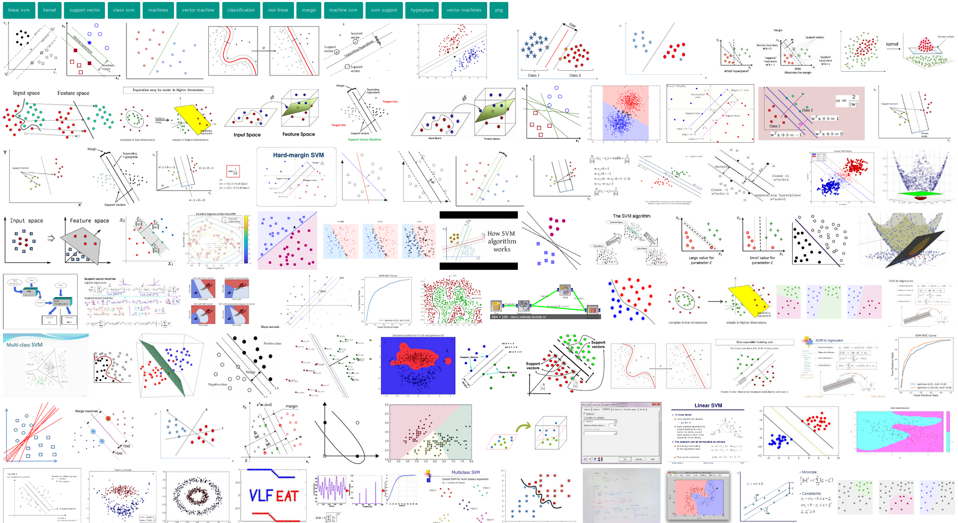
A support vector machine classifier or, in short, SVM classifier is computer method that aim to find the best hyperplanes that separate the classes, maximizing the largest separation (or margin) between the classes. Separation is usually linear but it can be generalized.
5. Examples with R
For the titanic dataset (survival binary classification), probably the best synthesis with a lot of known classifiers is here (with Python) though this other analysis is interesting (with R).
For the iris dataset (classification for three species), probably the best synthesis with a lot of known classifiers is here. An unsupervised version, available there is also very interesting.
Some more examples, by topics:
|  Retour à la page principale de
(gH)
